


You are here
An Implementation of Piecewise-Linear Interpolation for 3D Slice Reconstruction
In a winter 2008 course I took on select topics of medical computing (COMP 5308), I chose to tackle an implementation for slice reconstruction as my project. This page contains excerpts from the accompanying paper I wrote.
Introduction
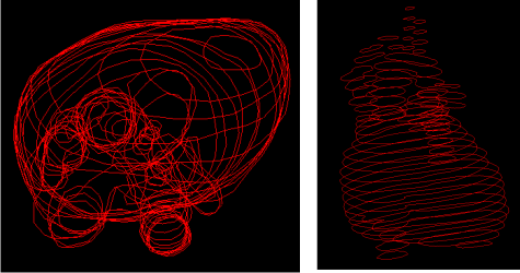
In the world of medical computing, 3D reconstruction of slice data is a common topic. A slice is a single cross-section image obtained by CT or MRI devices, and can be processed to obtain polygonal data describing the material to be analyzed. For example, if images are taken of a heart, contours around the cross sections might be found and saved as point data for further processing. An example of this is shown below. It is then possible to reconstruct these polygonal contours into a 3D object by connecting the appropriate pieces together.
This page details an implementation of the 3D reconstruction process from slices consisting of simple, non-overlapping polygonal contours using the methods of Gill Barequet and Micha Sharir in Piecewise-Linear Interpolation between Polygonal Slices.
Overview of the Implemented Algorithm
As mentioned, the method implemented in this paper is due to Gill Barequet and Micha Sharir. It was chosen for its relative simplicity and good results for handling more complicate geometries like branching. This section will briefly outline the algorithm, saving most of the detail for the implementation discussion.
The first step is to read and preprocess the slice data. Each polygonal contour must be listed as a cycle of points in three dimensions, and the z-coordinate must be the same for all contours on a slice. The contours must be listed in a consistent direction; for example, the convention that polygons listed in counter-clockwise order have their area situated in their interiors, whereas clockwise contours represent holes. For the preprocessing, each edge on the polygon is subdivided into several smaller edges of equal length, thereby discretizing the contours.
Next, each pair of adjacent slices is examined in search of contours that have matching portions. To accomplish this, each contour's cycle of edges must be arbitrarily broken so polygonal chains are used instead. A voting process helps find potentially matching alignments between two chains, and possible matches are further processed to find their beginnings and ends. Overlap is eliminated and matches are filtered by a scoring system that assesses their quality. This process uses a predefined maximum distance value to determine whether two points match, and keeps only those matching chains that have more than one point. As a result, only contours with the same orientation (i.e. clockwise or counter-clockwise) will be matched.
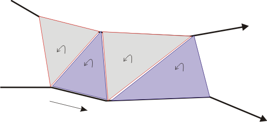
Those portions of contours that matched are now stitched together. That is, triangles are inserted along the chain, starting at one end and proceeding to the other. It is important to orient these triangles consistently; in the case that outer contours are listed in clockwise order, so should the triangles be. This is depicted below.
The nesting hierarchy is found for these cleft cycles, and then each group of outermost clefts and their children is used to create a complete graph. This graph will have one node for each cleft cycle and edges connecting all nodes to each other node. A minimum spanning tree is then run on this graph. Edges are added between two cycles to bridge them together if the minimum spanning tree has an edge between the two nodes representing the cycles, thereby turning the group of clefts into one single cycle. This new polygon is then triangulated. The triangles from the stitched matches and these new triangles form the mesh for the reconstruction, along with the top and bottom slice to cap off the object on either end.
Implementation Details
The C++ code for this project was developed in Visual Studio using OpenGL, OpenGL Utility, and GLUT libraries. The software ran with reasonable running times on a laptop with a 1.79 GHz AMD processor and 512 MB of RAM. The remainder of this section will outline the main classes involved and how the algorithm was specifically implemented.
The following classes form the core of the implementation:
- Contour
- Slice
- SliceArray
- Triangle and Polyhedron
- Cleft and CleftEdgeCycle
The contour class stores a vector of three-dimensional points representing a polygonal chain. This class is responsible for computing and filtering the match candidates between two contours. It has an inner public class called MatchCandidate that stores pointers to the two contours involved in a match, and the match start and end indexes from the contour's vector. A contour also knows how to render an outline of itself in an OpenGL environment.
The Slice class is essentially a sophisticated container for a set of contours. Most of what it can do it does by forwarding messages to the contours it stores. Its most complicated function is to read a file of slice data and store it in the appropriate format. Similarly, the SliceArray class acts as a container of slices.
The Triangle and Polyhedron classes are used to store the triangle mesh that is created during the matching process. The function buildPolyhedron takes a set of matches for two slices and performs the rest of the algorithm, eventually adding to its set of triangles. It, too, knows how to render itself in an OpenGL environment.
Finally, the Cleft class stores both endpoints of an edge. The reason for this will become clear in the algorithm discussion to follow. Meanwhile, the CleftEdgeCycle represents a full cycle of cleft edges, collectively known as a single cleft. It is able to find cycles within a set of cleft edges, as well as bridge a group of related cycles into one cycle.
There are other secondary classes in the project, used for the user interface (rendering and interaction) and triangulating the cleft cycles. Some of the code is due to (Arcball; Video Tutorials Rock; Tesselation).
The first major step is the initial search for match candidates. Although the method in (piecewise) using a voting system to find the most promising shifts, this implementation does not do so explicitly. Instead, a loop over all possible shifts between the two contours in question searches for chains with most points in close proximity that are long enough to be considered matches. The number of points examined for each of these shifts is the maximum length of the two contours involved. This means that one contour may loop around, but any issues with range are saved until later. For each of these points, the distance between their xy-projections is checked to see whether it is within the allowable range. If not, then the number of mismatches since the start of the current match chain is compared to the maximum allowed. If the points do not fulfill all this criteria, the current chain is terminated and a new one started. Otherwise, the current match chain continues. A series of mismatches before or after the chain will not be included in it.
Next, the matches found must be adjusted so there is no overlap. To accomplish this, the indexes in the MatchCandidate class conform to the following criteria: first, the start index of a match chain will be less than the number of points of its associated contour; second, the total number of points in the match will not exceed the minimum length of the two contours; and finally, the end index will not precede the start index. This means that the end index may extend past the number of points in a contour; this is intentional and will help sort out the overlaps. The matches will be put back into range later.
A match candidate will be given a list of other matches. Once adjusted to avoid overlapping with anything in the list, the match will be added to it (assuming it is not completely contained in the other matches). To check for overlap, both the upper and lower contour indexes must be checked. When comparing two matches for overlap, the following cases may occur, where 'this match' refers to the one to be added, and 'other match' refers to one from the list:
- This match is completely contained in the other match. This match will not be added to the list.
- The other match is completely contained in this match. Break this match into two, one before and one after the other match. Recursively check for overlap for the two pieces.
- This match begins before but overlaps the other match. Adjust the end of this match to come before the other match.
- This match begins after the start of the other match but overlaps it. Adjust the beginning of this match to come after the end of the other match.
- No overlap. No action is required in this case.
After the non-overlapping matches are each processed for triangle stitching, all triangle edges and contour edges are saved as cleft edges. As mentioned above, these edges are saved with both endpoints, so finding cycles among them will be simple. Starting with any random edge, the next edge in the cycle will start with the same point this edge ends with. If all edges are stored in a map data structure, keyed on their first endpoint, finding the next edge in the cycle is as simple as looking up the second endpoint in the map.
Groups of cycles are then determined using the Jordan curve theorem. A vertical ray starting at one contour is intersected with each edge of another contour. If there is an even number of intersections, the two contours are completely disjoint; otherwise, they belong to the same group.
After the complete graph is computed for each of these groups, Prim's minimum spanning tree algorithm is used to determine where the cycles should be branched to other cycles in the group. To do the actual bridging, a random cycle is traversed from the first edge until a bridging edge is reached. Each edge is added to a new cycle. The function recursively walks around the other cycle, starting from the bridging point. When it returns, the rest of the first cycle is added to the new one. The algorithm ends by triangulating the new cycle.
Results
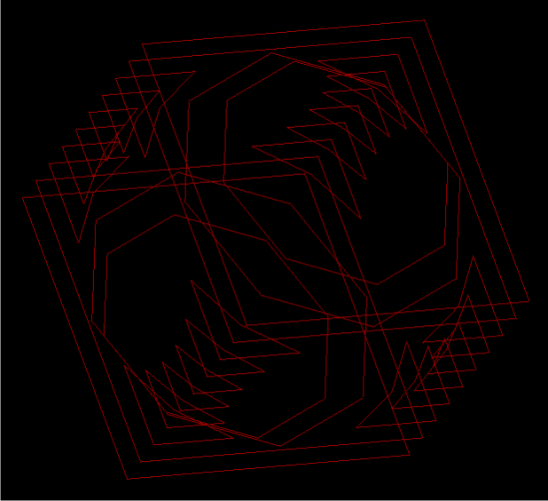
Data of a cube with a circular hollow was used to test that the implementation works on a basic level. Some slice pairs contained the same contours, which matched perfectly in the implementation. There is some complicated geometry for some of the inner corners in the model, since part of these small, triangular shaped contours needed to match with the corners above them, and part needed to match with the cube's square boundary. The image below shows the slices of the cube, viewed from an angle.
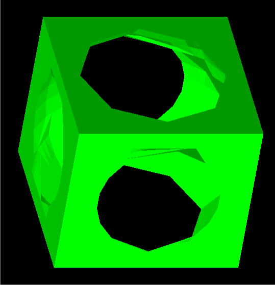
The cube was reconstructed with no problems; that is, the whole solid was recreated without any holes. The results can be seen below.
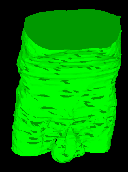
The next example data was that of a male torso. It did not fare quite as well as the cube, having a few holes here and there. Regardless, there are no major problems, and situations of branching were indeed handled. The reconstruction is shown below.
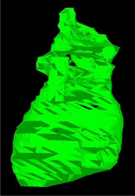
Finally, the heart whose slices were shown at the top are shown reconstructed below. This model obviously did not fare as well as the previous two, with more holes and more instances of unnatural connections between several slices.
Conclusion
Based on the results of the hollowed out cube, the algorithm is implemented reasonably well. However, some of the aspects of the implementation were very tricky, and could have easily resulted in small bugs that may lead to the holes and seen in the torso and heart. The quality of the heart reconstruction compared to the cube, on the other hand, seems to suggest that there are still limitations to this method. Indeed, if it were perfect, there would not have been so many subsequent papers written on the topic in the last decade or so. Even with these limitations, this method is relatively simple, and has much promise for use in practical applications that don't involve complex data.
Project Paper
Download the project paper in PDF.